This post was written by Sacha Epskamp.
Tomorrow our biannual network school will start again (see here for last year’s materials), which is also the time I update all software packages on CRAN. Most notably, I have updated bootnet to version 1.3 and psychonetrics to version 0.5. Given that it is now easier to reproduce results from older version through the checkpoint package, I have decided to change some default behavior that was more harmful than good (see also here for my thoughts on changing defaults and a checkpoint example). To this end, you may obtain different results with these new versions, although old behavior should be perfectly mimicked by setting the right arguments. Below, I will describe some of the most prominent new features and changes.
Changes in bootnet version 1.3
Handling of Missing Data
Previous default behavior
Several of the most commonly used default estimators in bootnet (e.g., EBICglasso, ggmModSelect, and pcor) rely on a correlation matrix as input, which is computed in the estimateNetwork function. When data are missing, such an input correlation matrix can not be computed directly. The default behavior was to then instead compute correlations pairwise. While this works (as it leads to a network without errors), pairwise estimation does come with a complication: the network estimation routines also require a sample size (e.g., for the BIC computation). This was controlled with the sampleSize argument, which had only two options: maximum (the old default), which simply set the sample size to all rows in the data, and minimum, which set the sample size to the number of rows that had no missing data at all. To understand why these are both problematic, consider the following dataset:
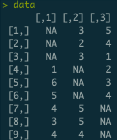
In this dataset, there are three variables (columns), nine cases (rows). Some of the data are missing: only six observations are available per variable and only two observations are available per case. We can use pairwise estimation to compute the input correlation matrix:
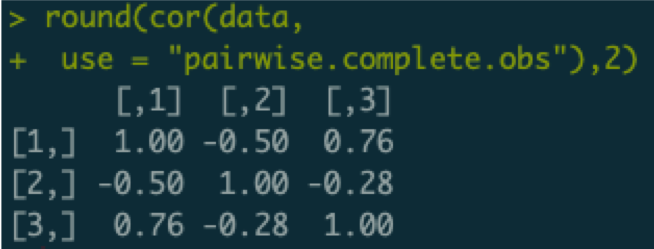
Of note, each element in this correlation matrix is only based on three observations. For example, the correlation between variables two and three is only based on the data of the first three cases who do not have missing values on either variable 1 or 2. If we now set the sample size to the maximum (the old default), we would subsequently estimate a network thinking we have nine observations. This would be problematic, as we would severely overestimate how confident we are about these correlations, and subsequently may include false edges in our network. If we would use the minimum sample size, we are left with a sample size of zero, which would underestimate our confidence (plus likely lead to some errors).
New default behavior
In the new version of bootnet, three more options are added: pairwise_average (the new default), pairwise_minimum, and pairwise_maximum. These set the sample size to the average, minimum, or maximum sample size used for each individual correlation. In this case, all three options would set the sample size to three, which is a much better description of the data. Simulation studies I am performing together with Adela Isvoranu indicate that these options provide a much more balanced performance of network estimation when data are missing (provided each variable has about the same amount of missingness).
Of note, technically using a pairwise correlation matrix as input to a likelihood based method (e.g., EBICglasso, ggmModSelect, and pcor) is not correct. This is because the likelihood function of the multivariate Gaussian only becomes a function of the summary statistics (means, variances and covariances) when no data is missing. All these methods compute the likelihood based on the input summary statistics, and hence even though performance is ok using a pairwise correlation matrix does not return the correct likelihood. A more technically sound method of dealing with missings is to compute the likelihood per case or per block of observed data with the same missingness pattern. One such a method is full information maximum likelihood (FIML) estimation, which already is included in psychonetrics. For confirmatory fit, FIML is recommended over pairwise estimation of the input correlations. For exploratory search, the algorithms in bootnet tend to perform a bit better at lower sample sizes than the algorithms included in psychonetrics, but FIML will start outperforming at larger sample sizes.
Other changes in bootnet 1.3
Beyond the sample size change, there are a few additional changes in the new version of bootnet:
- Several estimators now support the argument corMethod = “spearman”, which will make it much easier to use Spearman correlations instead of polychoric correlations as input to some of the estimators. A future version of bootnet may make this default behavior.
- Ever since the release of the first paper on bootnet, the intended method of specifying a custom estimator function was by supplying a custom function to the fun argument. Before this, I had another more complicated method implemented, using arguments such as graphFun, and estFun. These were not really used and are now no longer supported.
- The help file of estimateNetwork also lists the functions used as default function for the fun argument. For example, default = “EBICglasso” sets the function bootnet_EBICglasso to the fun argument, allowing you to use any argument from bootnet_EBICglasso in estimateNetwork. These default functions themselves, however, are not intended to be used manually (as is explained in the help file). Because many people do use these manually, the new version of bootnet will simply return an error if such a function (e.g., bootnet_EBICglasso) is used directly. This can be overwritten with unlock = TRUE, though that is not recommended.
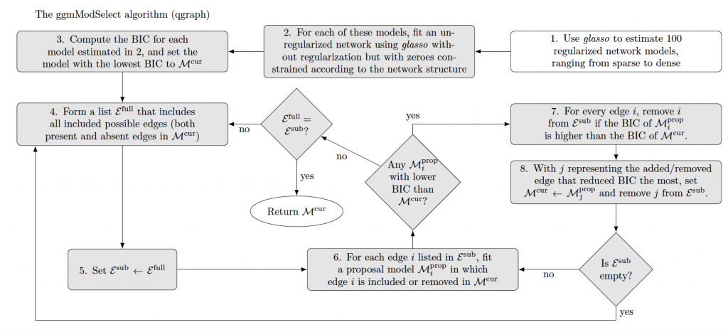
The ggmModSelect Algorithm
While not really a change in bootnet, I recently made a figure explaining the increasingly commonly used ggmModSelect algorithm in qgraph and bootnet:
Changes in psychonetrics version 0.5
Some of these changes also include changes in the earlier released version 0.4. Note that this blog post describes version 0.5.1, which is currently submitted to CRAN but may not yet be updated.
New modelsearch algorithm
Inspired by the ggmModSelect algorithm explained above, the new version of psychonetrics now contains a variant of this algorithm that makes use of significance levels and modification indices. This algorithm is implemented in the modelsearch function in psychonetrics, and works as follows:
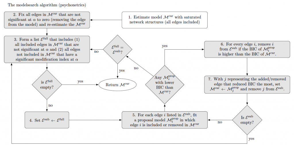
The algorithm is explained in more detailed and evaluated in simulation studies in the updated pre-print on latent network modeling with time-series and panel data. Generally it performs well in retrieving the network structure, being more sensitive than other algorithms in psychonetrics while retaining high specificity. Of note, however, is that just like the ggmModSelect algorithm the algorithm relies on many model evaluations and can be very slow with larger network models (e.g., more than 20 nodes). While the model is faster than ggmModSelect in theory (less model evaluations needed), it is currently slower in practice due to psychonetrics being slower than glasso in fitting given network structures.
Code example of the modelsearch algorithm
An example of the algorithm is below:
# Load libraries:
library("bootnet")
library("psychonetrics")
library("qgraph")
library("dplyr")

# Random seed:
set.seed(1)

# Construct a network
truenet <- genGGM(12)

# Generate data:
data <- ggmGenerator()(500, truenet)

# ggm model:
mod <- ggm(data)

# Estimate model:
mod <- mod %>% prune %>% modelsearch

# Obtain network:
estnet <- getmatrix(mod, "omega")

# Plot results:
layout(t(1:2))
qgraph(truenet, title = "True network", theme = "colorblind")
qgraph(estnet, title = "Estimated network", theme = "colorblind")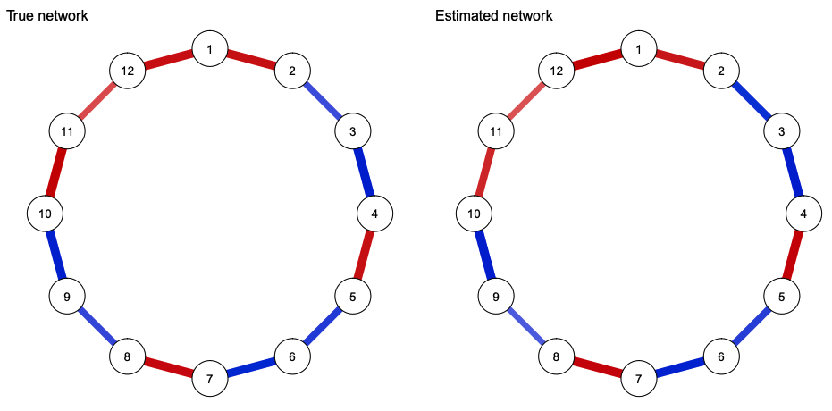
Maximum Likelihood Covariances as Input
All models in psychonetrics can be estimated using a variance-covariance matrix as input. Previously, a confusing aspect of psychonetrics was that it expected a maximum likelihood (ML) estimate of the variance-covariance matrix (denominator n), while the default R function cov returns an unbiased (UB) estimate of the variance-covariance matrix (denominator n-1).
Three changes in psychonetrics now simplify this behavior. First, the covML function can be used to obtain a ML variance-covariance matrix, and the functions covUBtoML and covMLtoUB can be used to transform between ML and UB estimates. Second, all models now contain the argument covtype, which can be specified to determine which type of input covariances were used (if covtype = “UB” the input variance-covariance matrix will be transformed). This allows you to use the UB estimates from the base R cov function in the input as well. Finally, if covtype is not specified psychonetrics will make an educated guess by seeing if UB or ML estimates are more likely to result from integer valued input data (as many psychological datasets are encoded using only integers).
For example, we can replicate the above analysis exactly using the input means and covariances:
# means:
means <- colMeans(data)

# UB covs:
covmat <- cov(data)

# ggm model:
mod2 <- ggm(means = means, covs = covmat,
covtype = "UB", nobs = 500)

# Estimate model:
mod2 <- mod2 %>% prune %>% modelsearch

# Show these are equal:
compare(rawdata = mod, summary = mod2)
# Gives identical fit
Correlations as input
Already included in version 0.4, psychonetrics now supports having a correlation matrix as input. Typically, correlation matrices are treated as variance-covariance matrices in network estimation (e.g., this is what EBICglasso and ggmModSelect do), which leads to minimal problems but is technically not correct. The reason this is not correct is that the variances are also estimated, while these are already known to be exactly 1 in correlations. Hence, not taking precautions when using correlations as input to an estimator that expects a variance-covariance matrix can lead to some biases, such as incorrect standard errors. The varcov family of psychonetrics now supports using a correlation matrix as input through the argument corinput = TRUE, in which case the variances are not estimated but determined from the network structure. Future updates will also bring this argument to other model families. In the example above, the following code can be used to obtain the same network structure:
# Correlation estimate
cormat <- cor(data)

# ggm model:
mod3 <- ggm(
     covs = cormat,
     corinput = TRUE,
     covtype = "ML", # <- not needed in 0.5.1
     nobs = 500)
Note that in this model, only network parameters are estimated and no means or scaling parameters are included (meanstructure = FALSE):
> mod3 %>% parameters

 Parameters for group fullsample
	-  omega (symmetric)
 var1 op var2   est    se        p row col par
   V2 --   V1 -0.35 0.032 < 0.0001   2   1   1
  V12 --   V1 -0.39 0.032 < 0.0001  12   1   2
   V3 --   V2  0.32 0.033 < 0.0001   3   2   3
   V4 --   V3  0.38 0.031 < 0.0001   4   3   4
   V5 --   V4 -0.38 0.031 < 0.0001   5   4   5
   V6 --   V5  0.29 0.033 < 0.0001   6   5   6
   V7 --   V6  0.36 0.032 < 0.0001   7   6   7
   V8 --   V7 -0.38 0.032 < 0.0001   8   7   8
   V9 --   V8  0.24 0.034 < 0.0001   9   8   9
  V10 --   V9  0.38 0.033 < 0.0001  10   9  10
  V11 --  V10 -0.32 0.034 < 0.0001  11  10  11
  V12 --  V11 -0.25 0.035 < 0.0001  12  11  12
WLS estimation of ordered data
Many datasets used for network estimation contain ordered categorical data (e.g., 4 point liker scale data), for which no good methods currently exist. A common way of handling this type of data, which I also suggested earlier, is to use polychoric correlations rather than Pearson correlations, as is typical in structural equation modeling (SEM) literature. While polychoric correlations are much better at estimating the correlation between two ordered categorical variables, using them as input in likelihood based network estimation routines (e.g,. EBICglasso and ggmModSelect) does pose several problems. Mainly, polychoric correlations are potentially very unstable as indicated by bootstrapped confidence intervals. This is a problem because the likelihood based method assumes the input correlations are Pearson correlations, which are much more stable, and hence using polychoric correlations can overestimate the confidence in correlations, compounding in overconfidence in the network structure. In fact, using polychoric correlations as input to a likelihood based method is technically wrong as the likelihood derived using polycoric correlations is not equal to the true likelihood of the data, much like the case with pairwise estimates above.
Because of this reason, it is typical for SEM analyses to not use maximum likelihood estimation but rather weighted least squares (WLS) estimation when analyzing ordered categorical data using polychoric correlations. This has been outlined decades ago in a classical paper by Bengt Muthén, but was so far not extended to network estimation routines. I have now implemented WLS estimation for GGM models in psychonetrics, and hope to extend this to all other model families soon. WLS estimation more appropriately adjusts standard errors to account for instability in the polychoric correlations, and therefore leads to more conservative estimators. Another benefit of WLS estimation is that it can naturally handle missing data through pairwise estimation (standard errors are automatically properly adjusted). The downside, however, is that WLS estimation seems to be very conservative and requires much larger datasets (e.g., thousands of cases) to reliably estimate network structures (especially when these are dense). Me and Adela Isvoranu are currently investigating the performance of WLS estimation in large-scale simulation studies.
To use WLS estimation of ordered categorical data in psychonetrics, simply use ordered = TRUE and missing = “pairwise” in the varcov model family:
# Generate data:
data <- ggmGenerator(ordinal = TRUE, nLevels = 3)(500, truenet)

# ggm model:
mod4 <- ggm(data, ordered = TRUE, missing = "pairwise")
The Ising Model
This year marks the 100th year since the Ising model was originally invented by Wilhelm Lenz, and what better way to celebrate this occasion by implementing the Ising model in psychonetrics? In version 0.5 the Ising distribution is now included as first distribution besides the Gaussian distribution. The function Ising can be used to specify the Ising model, the first model that uses this distribution (and which is simply identical to the distribution). Future versions of psychonetrics will likely see other models using this distribution (such as the FLaG-IRT model).
Important aspects of the Ising model implementation
Some important things to note are:
- Currently only maximum likelihood is supported, which requires the computation of the expensive partition function. To this end, the Ising model is currently only practically useable up to 20 nodes or so.
- The input matters, as any form of dichotomous data can be used (e.g., 0 and 1 encoding or -1 and 1 encoding), leading to structurally different models and parameter interpretations (the models will no longer be equivalent in multi-group settings).
- Just like Gaussian models, the model is actually fitted to the pairwise summary statistics (means and sums of squares). This means that all fit measures are also comparing the fitted Ising model to a ‘saturated’ Ising model in which all edges are present, similar to how GGMs and SEM models are fitted. This marks a departure from how such a model would be evaluated in typical loglinear modeling settings. The Ising model is equivalent to a loglinear model with only pairwise interactions, and such a model would typically be compared to a saturated model that also includes higher order interactions. A future version of psychonetrics will also include these fit indices.
Ising model estimation example
The following code gives an example of Ising estimation:
# Load libraries:
library("psychonetrics")
library("qgraph")
library("dplyr")
library("IsingSampler")
library("igraph")

# Random seed:
set.seed(1)

# Construct a network
truenet <- 0.25 * as.matrix(get.adjacency(watts.strogatz.game(1,12,1,0)))

# Generate data:
data <- IsingSampler(1000, truenet, rep(0, 12), responses = c(-1, 1))

# Ising model:
mod5 <- Ising(data)

# Estimate model:
mod5 <- mod5 %>% prune %>% modelsearch

# Obtain network:
estnet <- getmatrix(mod5, "omega")

# Plot results:
layout(t(1:2))
qgraph(truenet, title = "True network", theme = "colorblind")
qgraph(estnet, title = "Estimated network", theme = "colorblind")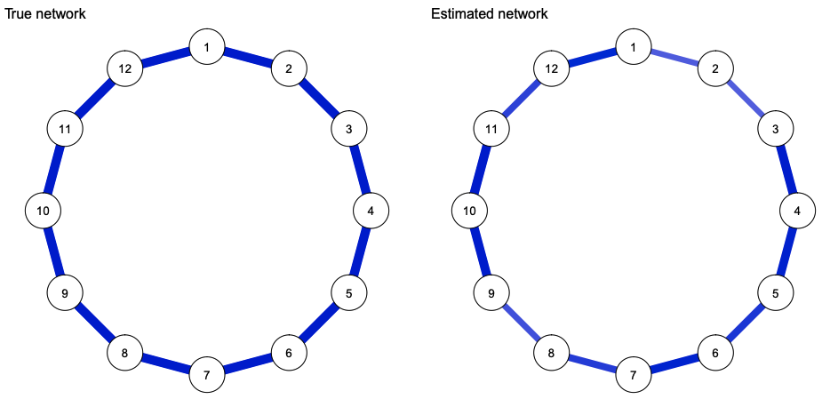
Fitting an Ising model to summary statistics
A benefit of the Ising model implementation in psychonetrics is that the model can be fitted to summary statistics (means and covariances), as long as these are derived from dichotomous data. For example, the following code uses the means, and variance-covariance matrix as input (note, this gives a bug in 0.5.0, but is fixed in 0.5.1):
# Means:
means <- colMeans(data)

# Covariances:
covmat <- cov(data)

# Ising model:
mod6 <- Ising(means=means, covs=covmat, responses = c(-1,1), nobs = 1000)

# Estimate model:
mod6 <- mod6 %>% prune %>% modelsearch

# Compare models:
compare(
  rawdata = mod5,
  summarystatistics = mod6
)
# These models are identical!
Multi-group models and temperature estimation
Like the Gaussian models, the Ising model implementation in psychonetrics allows for multgroup models. An extra use of this comes in the form if estimating the inverse temperature parameter (beta), which is typically constrained to 1 to identify the model parameters (this is the case in, for example, the IsingFit, IsingSampler, and mgm packages, which do not estimate a beta parameter at all). The beta parameter is very important in theoretical work however. For example, the stellar dissertation of Jonas Dalege uses the beta parameter to model attention, hypothesizing that people more familiar with the attitude object will feature a similar attitude network structure as people less familiar with the attitude object, but with a higher beta (lower temperature, indicating a reduction in entropy).
Using a multigroup analysis, the beta parameter becomes identified in each group beyond the first after placing equality constrains on the network and/or threshold parameters (much like variances of latent variables becoming identified in a multigroup SEM). To exemplify this functionality, and as a surprise for Jonas Dalege’s PhD defense, I gathered data online and among friends and colleagues of Jonas Dalege on ten dichotomous (yes/no) attitude items. This data is included in psychonetrics as the dataset Jonas. Code to reproduce the analysis are in the help file of the Ising function, as well as below:
library("psychonetrics")
library("dplyr")

# Load dataset:
data("Jonas")

# Variables to use:
vars <- names(Jonas)[1:10]

# Arranged groups to put unfamiliar group first (beta constrained to 1):
Jonas <- Jonas[order(Jonas$group),]

# Form saturated model:
model1 <- Ising(Jonas, vars = vars, groups = "group")

# Run model:
model1 <- model1 %>% runmodel

# Prune-stepup to find a sparse model:
model1b <- model1 %>% prune(alpha = 0.05) %>%  stepup(alpha = 0.05)

# Equal networks:
model2 <- model1 %>% groupequal("omega") %>% runmodel

# Prune-stepup to find a sparse model:
model2b <- model2 %>% prune(alpha = 0.05) %>% stepup(mi = "mi_equal", alpha = 0.05)

# Equal thresholds:
model3 <- model2 %>% groupequal("tau") %>% runmodel

# Prune-stepup to find a sparse model:
model3b <- model3 %>% prune(alpha = 0.05) %>% stepup(mi = "mi_equal", alpha = 0.05)

# Equal beta:
model4 <- model3 %>% groupequal("beta") %>% runmodel

# Prune-stepup to find a sparse model:
model4b <- model4 %>% prune(alpha = 0.05) %>% stepup(mi = "mi_equal", alpha = 0.05)

# Compare all models:
compare(
  `1. all parameters free (dense)` = model1,
  `2. all parameters free (sparse)` = model1b,
  `3. equal networks (dense)` = model2,
  `4. equal networks (sparse)` = model2b,
  `5. equal networks and thresholds (dense)` = model3,
  `6. equal networks and thresholds (sparse)` = model3b,
  `7. all parameters equal (dense)` = model4,
  `8. all parameters equal (sparse)` = model4b
) %>% arrange(BIC) %>% select(model, DF, BIC)
In line with the predictions, a sparse network with equal network and threshold parameters but different beta parameters fits best (according to BIC). Further in line with the prediction, the group familiar with Jonas featured a lower temperature (higher beta parameter):
# Extract beta:
beta <-  unlist(getmatrix(model3b, "beta"))

# Standard errors::
SEs <- model3b@parameters$se[model3b@parameters$matrix == "beta"]

# Make a data frame:
df <- data.frame(
  temperature = 1/beta,
  group = names(beta),
  lower = 1 / (beta-qnorm(0.975) * SEs),
  upper = 1 / (beta+qnorm(0.975) * SEs),
  stringsAsFactors = FALSE
)

# Some extra values:
df$fixed <- is.na(df$lower)
df$group <- factor(df$group, levels = c("Doesn't know Jonas", "Knows Jonas"))

# Create the plot:
library("ggplot2")
g <- ggplot(df,aes(x=as.numeric(group), y = temperature, ymin = lower, ymax = upper)) +
  geom_line() +
  geom_errorbar(width = 0.05) +
  geom_point(cex = 5, colour = "black") +
  geom_point(aes(colour = fixed), cex = 4) +  theme_bw()  +
  xlab("") + ylab(expression(paste("Temperature (",1/beta,")"))) +
  scale_x_continuous(breaks =  1:2, labels = levels(df$group), expand = c(0.1,0.1)) +
  scale_y_continuous(expand = c(0,.1), limits = c(0,1)) +
  theme( panel.grid.major.x = element_blank(),panel.grid.minor.x = element_blank())+
  ggtitle(expression(paste("Model 6: 2 groups; ",bold(Omega)," sparse & equal; ",bold(tau)," equal; ",beta," free"))) +
  scale_colour_manual(values = c("black","white")) +
  theme(legend.position = "none")

# Plot:
print(g)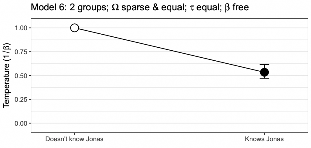
Finally, the estimated network structure can also be retrieved:
# Make labels:
labels <- c("good scientist",
            "wears beautiful\njeans",
            "cares about\npeople like you",
            "solve economics",
            "hardworking",
            "honest",
            "in touch with\nordinary people",
            "knowledgeable",
            "can't make up\nhis mind",
            "gets things done")

# Extract network structure and thresholds:
network <- getmatrix(model3b, "omega")[[1]]
thresholds <- getmatrix(model3b, "tau")[[1]]

# Scale thresholds for colors:
scaledthresh <- as.vector(thresholds / (2*max(abs(thresholds))))

# Make colors:
cols <- ifelse(scaledthresh < 0, "red", "darkblue")
cols[scaledthresh>0] <- qgraph:::Fade(cols[scaledthresh>0],alpha = scaledthresh[scaledthresh>0], "white")
cols[scaledthresh<0] <- qgraph:::Fade(cols[scaledthresh<0],alpha = abs(scaledthresh)[scaledthresh<0], "white")

# Plot network and save to file:
qgraph(network, layout = "spring", labels = labels,
            shape = "rectangle", vsize = 15, vsize2 = 8,
            theme = "colorblind", color = cols,
            cut = 0.5, filetype = "png", filename = "Jonas",
            repulsion = 0.9)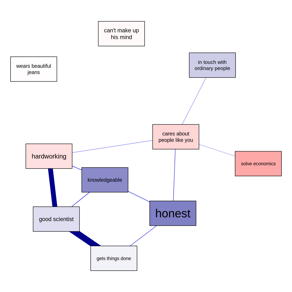
Of note, however, this analysis is very preliminary, and we are still working out the best way in which such multigroup Ising model analyses could be performed. If you have any thoughts for improvement, please let me know!
Concluding comments
This blog post described some new functionality in the bootnet and psychonetrics R packages. If you encounter any problems or if you have other suggestions, please submit these to the Github pages of bootnet and psychonetrics.