Simulation studies in R with the ‘parSim’ package

(featuring missing data analysis)

Simulation studies are absolutely vital for methodological work to be validated and tested in multiple settings. One simulation study is good, but more simulation studies are always better. In the context of network estimation for example, simulation studies are currently the only way to go in assessing the sample size needed, and a simulation study varying new conditions pointed out crucial problems in network estimation practices. Writing a simulation study in R is not very hard, but can take some time to set up.

My approach used to be to put all my simulation conditions in expand.grid to create a big data frame with conditions, then loop over this data frame to perform my simulations, storing the results in a new data frame, and finally left_join the results to have a big overview of simulation results.

I wrote the same code over and over again, and figured it would be easier to write a function to do this. I ended up using the function over and over again, and figured it might as well be an R package. This ended up as the very small and simple parSim package, which only contains a single function. I have written some examples on this on the Github page.

This blog post will exemplify how to use parSim for your own research!

Simple example: regression analysis

Let’s start with a very simple example. Suppose I have two variables: x and y, and the true linear regression relationship between these takes the following form:

Y = 0.5 * X + error

Thus, in a regression analysis there is no intercept (beta0 = 0) and only one slope (beta1 = 0.5). We can simulate this in R:

sampleSize <- 500
trueBeta <- 0.5
set.seed(123)
X <- rnorm(sampleSize)
Y <- trueBeta * X + rnorm(sampleSize)

Next, we can run a regression analysis and obtain estimates for the intercept and the slope:

fit <- lm(Y ~ X)
coefs <- coef(fit)
coefs

##   (Intercept)             X 
## -0.0004677688  0.4460270974

Let’s suppose we are interested in the absolute bias between our estimates and the true values. We can compute these as follows:

# Intercept bias (beta0 = 0):
interceptBias <- abs(coefs[1])

# Slope bias:
slopeBias <- abs(coefs[2] - trueBeta)

Finally, we can store these in a nice list to keep the results contained:

Results <- list(
  interceptBias = interceptBias,
  slopeBias = slopeBias
)

Performing the simulations in parSim

Using the parSim package in general takes the following form:

library("parSim")

parSim(

  # << ENTER SIMULATION CONDITIONS HERE >>

  reps = # << NUMBER OF REPITITIONS >>,
  write = # << TRUE/FALSE >>,
  name = # << NAME OF THE SIMULATION STUDY >>,
  nCores = # << NUMBER OF CORES TO USE >>,
  expression = {

    # << ENTER SIMULATION CODE HERE>>

    # << OUTPUT MUST BE LIST OR DATA FRAME >>>  
  }
)

The write argument will control if we return results to an object (as data frame) or write them to a text file. Let’s set this to TRUE to store our results (the name argument will be used for the filename). The reps argument controls how many repetitions you want per condition. For testing purposes, set this to 2 or 10 or so, and when you are happy with your setup you can increase this to 100 or even higher. The nCores argument controls how many computer cores are used. If this is higher than 1, you need to load packages in the simulation code. I recommend leaving this to 1 for testing purposes, and only increasing the number if you are confident about your simulation setup.

The way parSim mainly works is that we assign simulation conditions in the function as argument, and then can use the same names in the R expression. That is, if I enter:

sampleSize = c(50, 100, 250, 500, 1000)

in the simulation conditions, I can use the object sampleSize in the simulation code! It will be varied between 50, 100, 250, 500, and 100 then. The output must be a list, or a data frame with a row for additional conditions (e.g., if I want to compare two estimation procedures). This means that we can easily use our code above in parSim:

library("parSim")

parSim(
  ### SIMULATION CONDITIONS
  sampleSize = c(50, 100, 250, 500, 1000),

  reps = 100, # 100 repititions
  write = TRUE, # Writing to a file
  name = "parSim_regression", # Name of the file
  nCores = 1, # Number of cores to use
  expression = {
     # True beta coefficient (random):
    trueBeta <- rnorm(1)

    # Generate data:
    X <- rnorm(sampleSize)
    Y <- trueBeta * X + rnorm(sampleSize)

    # Run analysis:
    fit <- lm(Y ~ X)

    # Store coefficients:
    coefs <- coef(fit)

    # Intercept bias (beta0 = 0):
    interceptBias <- abs(coefs[1])

    # Slope bias:
    slopeBias <- abs(coefs[2] - trueBeta)

    # Results list:
    Results <- list(
      interceptBias = interceptBias,
      slopeBias = slopeBias
    )

    # Return:
    Results
  }
)

The function wrote a file I can read:

table <- read.table("parSim_regression.txt", header = TRUE)

which contains a simulation condition per row:

head(table)

##   sampleSize rep id interceptBias   slopeBias error errorMessage
## 1       1000  45  1   0.004440148 0.038575289 FALSE           NA
## 2       1000  51  2   0.014662430 0.007679153 FALSE           NA
## 3        500  10  3   0.016685096 0.019276944 FALSE           NA
## 4        500  87  4   0.028294452 0.038963745 FALSE           NA
## 5        100   9  5   0.041550819 0.090290917 FALSE           NA
## 6        100  92  6   0.029564444 0.015805679 FALSE           NA

I can easily use this with dplyr, tidyr and ggplot2:

library("ggplot2")
library("dplyr")
library("tidyr")

# Gather results:
table_gather <- table %>% gather(measure,value,interceptBias:slopeBias)

# Plot:
ggplot(table_gather, aes(x=factor(sampleSize), y=value, fill = measure)) + 
  geom_boxplot(outlier.size = 0.5,lwd=0.5,fatten=0.5) + 
  xlab("Sample Size") + 
  ylab("") + 
  theme_bw() + 
  theme( panel.grid.major.x = element_blank(),panel.grid.minor.x = element_blank()) +
  geom_vline(xintercept=seq(1.5, length(unique(table_gather$sampleSize))-0.5, 1),
             lwd=0.5, colour="black", alpha = 0.25) 

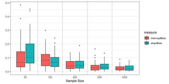
This nicely shows that the bias in parameter estimation goes down as a function of sample size!

Detailed example: network estimation with missing data

This being the psychonetrics blog, it would be the more logical to investigate the network estimation performance using psychonetrics rather than the performance of the lm function. Let’s investigate something that is actually quite a new topic of research: missing data analysis. To start, we need to generate data. We can use the bootnet package to generate a “true” network to simulate data under:

set.seed(123)
library("bootnet")
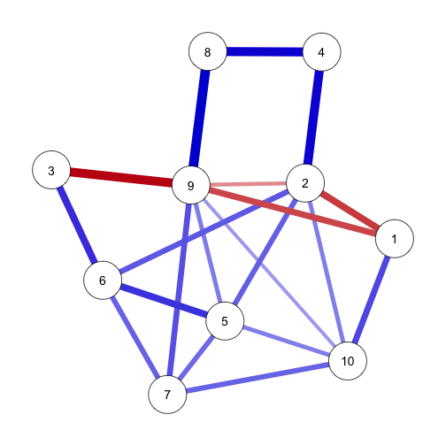
trueNet <- genGGM(10, nei = 2, propPositive = 0.8, p = 0.25)

This network consists of 10 nodes, with mostly positive edges and not unlike we see in the literature some times:

library("qgraph")
graph <- qgraph(trueNet, layout = "spring", theme = "colorblind")

Next, we need to generate data. We can use the bootnet package again for this: the ggmGenerator function generates a data generating function (I know… it is a bit confusing):

sampleSize <- 500
generator <- ggmGenerator()
Data <- generator(sampleSize, trueNet)

Next, we can add some missing data (10\% missing completely at random):

missing <- 0.1
for (i in 1:ncol(Data)){
  Data[runif(sampleSize) < missing,i] <- NA
}

Now, we can estimate our Gaussian graphical model, using the full information maximum likelihood estimator (FIML) in psychonetrics. To do this, we first need to create a model:

library("psychonetrics")
library("dplyr")
mod <- ggm(Data, estimator = "FIML")

This is a fully connected network model. It is not yet evaluated, so we need to run the model first:

mod <- mod %>% runmodel

Next, we can prune edges that are not significant. For example, we could use a false discovery rate (FDR) adjustment together with an alpha of 0.05. After pruning, psychonetrics will re-estimate the model, optimizing parameters taking into account that edges have been removed:

mod <- mod %>% prune(adjust = "fdr", alpha = 0.05, recursive = FALSE)

There are other ways to estimate a network, for example by using stepup to perform step-up estimation rather than step-down estimation, or by combining prune and stepup. A nice practice is to test out the differences between these algorithms in a simulation study yourself.

Now that we have a network model, we need to see if it is good. Let’s first retrieve it and plot it:

estNet <- getmatrix(mod, "omega")
graph <- qgraph(estNet, layout = graph$layout, theme = "colorblind")

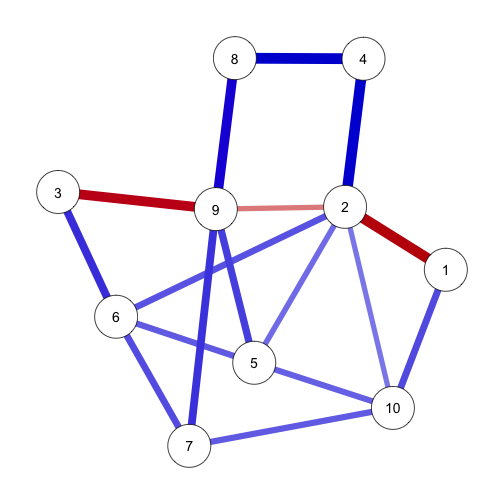
This looks quite similar to the original network, but it would be best to use some statistics for this. I often use a small function compareNetworks (available here) for this:

source("compareNetworks.R")
results <- compareNetworks(trueNet, estNet)
results[c("sensitivity", "specificity", "correlation")]

## $sensitivity
## [1] 0.85
## 
## $specificity
## [1] 1
## 
## $correlation
## [1] 0.9343398

We see that our estimation is highly conservative (high specificity), but also picks up many edges (moderate to high sensitivity) with a good correspondence between edge weights (moderate to high correlation). This is good! Let’s combine all these codes in a nicely contained code to run this simulation:

# Conditions:
sampleSize <- 500
missing <- 0.1

### Start simulation code ###
# Packages:
library("psychonetrics")
library("dplyr")
library("bootnet")

# Function needed:
source("compareNetworks.R")

# Generate true network:
trueNet <- genGGM(10, nei = 2, propPositive = 0.8, p = 0.25)

# Generate data:
generator <- ggmGenerator()
Data <- generator(sampleSize, trueNet)

# Add missings:
for (i in 1:ncol(Data)){
  Data[runif(sampleSize) < missing,i] <- NA
}

# Estimate model (FDR prune):
mod <- ggm(Data, estimator = "FIML") %>% 
  runmodel %>% 
  prune(adjust = "fdr", alpha = 0.05, recursive = FALSE)

# Extract network:
estNet <- getmatrix(mod, "omega")

# Compare to true network:
results <- compareNetworks(trueNet, estNet)

Pretty!

The resulting object results is already a list with values to return, so we don’t have to change much to this code to put it in parSim! The parSim code for performing this simulation study, varying sample size and missingness and repeating each condition 100 times (using 8 computer cores) is available here. It takes some time to run (about half an hour on a good computer for me). You can download results from this simulation study here if you do not want to wait for it to run.

Now, we can plot the results using the useful tidyverse packages again:

library("ggplot2")
library("dplyr")
library("tidyr")

# Read results:
table <- read.table("missingdata_sims_1.txt", header = TRUE)

# Label missings nicer:
table$missingFactor <- factor(table$missing, 
     levels = sort(unique(table$missing)),
     labels = paste0("Missingness: ",sort(unique(table$missing))))

# Gather results:
table_gather <- table %>% gather(measure,value,sensitivity:correlation)

# Plot:
ggplot(table_gather, aes(x=factor(sampleSize), y=value)) + 
   facet_grid(missingFactor ~ measure) + 
  geom_boxplot(outlier.size = 0.5,lwd=0.5,fatten=0.5) + 
  xlab("Sample Size") + 
  ylab("") + 
  theme_bw() + 
  theme( panel.grid.major.x = element_blank(),panel.grid.minor.x = element_blank()) +
  geom_vline(xintercept=seq(1.5, length(unique(table_gather$sampleSize))-0.5, 1),
             lwd=0.5, colour="black", alpha = 0.25) 

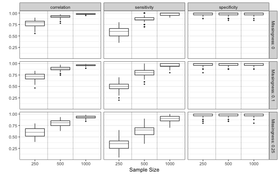
It seems that FIML estimation coupled with FDR pruning works very well for handling missing data!

We can extend our simulation study, and compare our results to, for example, mice imputation coupled with the ggmModSelect algorithm. The parSim code for such a simulation study is available here and results from a run on my computer are available here. Using almost the exact same code as above (I only set fill = method in aes()) gives the following results: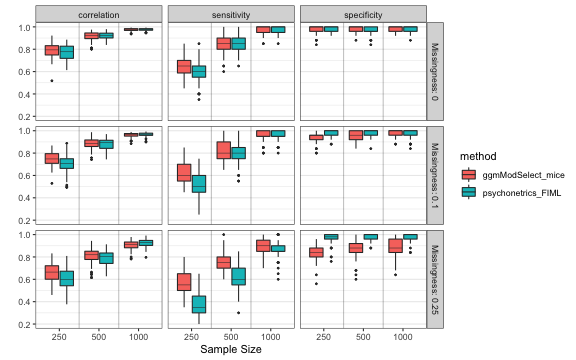

This clearly shows that ggmModSelect loses its specificity (detects more false edges) when we introduce missingness.

Tips for performing simulation studies

To conclude this blog post, here are some tips when setting up simulation studies:

• Debugging is easy. Just set nCores = 1 and put browser() somewhere in your code. Next, run the simulation study, and R will stop at the moment it encounters browser() and lets you look around in the simulation environment. Don’t know about browser()? It is probably the most incredible R function that exists! I use it almost every day!
• Be careful with how many conditions you put in. It is very alluring to vary everything you can, but every condition comes at a severe cost. For example, if I would vary also alpha between 0.01 and 0.05, my simulation would take twice as long! If I would add two more conditions with two levels each, it would take four times as long! Often, it is better to only really vary the thing you are interested in, and do not vary things that are too vague. For example, I never vary the number of nodes, as generating a network for 10 nodes is so different than generating a network for 20 nodes (e.g., edges must be weaker with more nodes to ensure positive definiteness), it is not clear what the real source of differences in results are (network density? power? computational feasibility?).
• Start simple, and move your way up from there. Start with 1 repetition on 1 core. Then try two cores. Then try more repetitions. It would be a shame to run a simulation for a day only to find out you made a small error in the code (this happened to me a lot).
• Be careful with interupting parallel processes. This does not work very well, and you might end up having some processes running in the background anyway. I sometimes had computers crashing from breaking a simulation study and starting one again. If you do have to break a parallel simulation study, it may be better to restart R or even your computer. Note, prevention is better here! Just start with nCores = 1, in which case interrupting works fine!
• Do not forget to load packages and source code when using multiple cores. If you set nCores > 1, a fresh R session is started for each simulation condition, which will not contain any objects from your current workspace (unless you use the parSim argument export). So you need to load packages and source .R scripts needed in the expression itself!
• Setting a random number generator seed does not work for multi-core simulations. Do not put set.seed() in the beginning of the expression as you would just repeat the exact same simulation over and over again. Setting it before the parSim call only works for nCores = 1. I haven’t implemented it yet for multi-core simulations (it doesn’t matter much, the general conclusion should not depend on the seed!).

That’s all for this blog post! Good luck with setting up your own simulation study!